Signal-flow graph

A signal-flow graph (SFG) is a special type of block diagram^[1]—and directed graph—consisting of nodes and branches. Its nodes are the variables of a set of linear algebraic relations. An SFG can only represent multiplications and additions. Multiplications are represented by the weights of the branches; additions are represented by multiple branches going into one node. A signal-flow graph has a one-to-one relationship with a system of linear equations.^[2] In addition to this, it can also be used to represent the signal flow in a physical system; i.e., it can represent relations of cause and effect.

1 Example 1: Simple amplifier
2 Example 2: Two-port network
3 Example 2a: Circuit containing a two-port network
4 Example 3 Asymptotic gain formula
5 Example 4: Position servo with multi-loop feedback
6 See also
7 Notes
8 References
9 External links

Example 1: Simple amplifier

The amplification of a signal V₁ by an amplifier with gain a₁₂ is described mathematically by

$V_2 = a_{12}V_1 \,.$

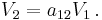
This relationship represented by the signal-flow graph of Figure 1. is that V₂ is dependent on V₁ but it implies no dependency of V₁ on V₂. See Kou page 57^[3].

Example 2: Two-port network

In electrical circuits, two equations describing a two-port network in admittance matrix form,

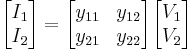
$\begin{bmatrix} I_1 \\ I_2 \end{bmatrix} = \begin{bmatrix} y_{11} & y_{12} \\ y_{21} & y_{22} \end{bmatrix} \begin{bmatrix} V_1 \\ V_2 \end{bmatrix}$

can be drawn as the SFG shown in Figure 2. This signal-flow graph describes causality properly if and only if V₁ and V₂ are designated as inputs. If any other designation of inputs is made then the SFG is either incomplete or invalid.

Example 2a: Circuit containing a two-port network

The figure to the right depicts a circuit that contains a two-port network. V_in is the input of the circuit and V₂ is the output. The two-port equations impose a set of linear constraints between its port voltages and currents. The terminal equations impose other constraints. All these constraints are represented in the SFG (Signal Flow Graph) below the circuit. There is only one path from input to output which is shown in a different color and has a gain of -R_Ly₂₁. There are also three loops: -R_iny₁₁, -R_Ly₂₂, R_inR_Ly₁₂y₂₁. Sometimes a loop indicates intentional feedback but it can also indicate a constraint on the relationship of two variables. For example, the equation that describes a resister says that the ratio of the voltage across the resister to the current through the resister is a constant which is called the resistance. This can be interpreted as the voltage is the input and the current is the output, or the current is the input and the voltage is the output, or merely that the voltage and current have a linear relationship. Virtually all passive two terminal devices in a circuit will show up in the SFG as a loop.

The SFG and the schematic depict the same circuit, but the schematic also suggests the circuit's purpose. Compared to the schematic, the SFG is awkward but it does have the advantage that the input to output gain can be written down by inspection using Mason's rule.

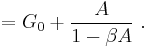
Example 3 Asymptotic gain formula

A possible SFG for the asymptotic gain model for a negative feedback amplifier is shown in Figure 3, and leads to the equation for the gain of this amplifier as

$G = \frac {y_2}{x_1}$ $= G_{\infty} \left( \frac{T}{T %2B 1} \right) %2B G_0 \left( \frac{1}{T %2B 1} \right) \ .$

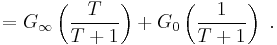
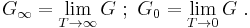
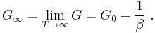
The interpretation of the parameters is as follows: T = return ratio, G_∞ = direct amplifier gain, G₀ = feedforward (indicating the possible bilateral nature of the feedback, possibly deliberate as in the case of feedforward compensation). Figure 3 has the interesting aspect that it resembles Figure 2 for the two-port network with the addition of the extra feedback relation x₂ = T y₁.

From this gain expression an interpretation of the parameters G₀ and G_∞ is evident, namely:

$G_{\infty} = \lim_{T \to \infty }G\�; \ G_{0} = \lim_{T \to 0 }G \ .$

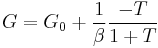
There are many possible SFG's associated with any particular gain relation. Figure 4 shows another SFG for the asymptotic gain model that can be easier to interpret in terms of a circuit. In this graph, parameter β is interpreted as a feedback factor and A as a "control parameter", possibly related to a dependent source in the circuit. Using this graph, the gain is

$G = \frac {y_2}{x_1}$ $= G_{0} %2B \frac {A} {1 - \beta A} \ .$

To connect to the asymptotic gain model, parameters A and β cannot be arbitrary circuit parameters, but must relate to the return ratio T by:

$T = - \beta A \ ,$

and to the asymptotic gain as:

$G_{\infty} = \lim_{T \to \infty }G = G_0 - \frac {1} {\beta} \ .$

Substituting these results into the gain expression,

$G = G_{0} %2B \frac {1} {\beta} \frac {-T} {1 %2BT}$

$= G_0 %2B (G_0 - G_{\infty} ) \frac {-T} {1 %2BT}$

$= G_{\infty} \frac {T} {1 %2BT} %2B G_0 \frac {1}{1%2BT} \ ,$

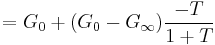
which is the formula of the asymptotic gain model.

Signal flow graphs are used in many different subject areas besides control and network theory, for example, stochastic signal processing.^[4]

Example 4: Position servo with multi-loop feedback

This example is representative of a SFG (signal-flow graph) used to represent a servo control system and illustrates several features of SFGs. Some of the loops (loop 3, loop 4 and loop 5) are extrinsic intentionally designed feedback loops. These are shown with dotted lines. There are also intrinsic loops (loop 0, loop1, loop2) that are not intentional feedback loops, although they can be analyzed as though they were. These loops are shown with solid lines. Loop 3 and loop 4 are also known as minor loops because they are inside a larger loop.

The forward path begins with $\theta_C \,$ , the desired position command. This is multiplied by K_P which could be a constant or a function of frequency. K_P incorporates the conversion gain of the DAC and any filtering on the DAC output. The output of K_P is the velocity command $V_{\omega C} \,$ which is multiplied by K_V which can be a constant or a function of frequency. The output of K_V is the current command, V_IC which is multiplied by K_C which can be a constant or a function of frequency. The output of K_C the amplifier output voltage, V_A. The current, I_M, though the motor winding is the integral of the voltage applied to the inductance. The motor produces a torque, T, proportional to I_M. Permanent magnet motors tend to have a linear current to torque function. The conversion constant of current to torque is K_M. The torque, T, divided by the load moment of inertia, M, is the acceleration, $\alpha \,$ , which is integrated to give the load velocity $\omega \,$ which is integrated to produce the load position, $\theta_L \,$ .

The forward path of loop 0 asserts that acceleration is proportional to torque and the velocity is the time integral of acceleration. The back ward path says that as the speed increases there is a friction or drag that counteracts the torque. Torque on the load decreases proportionately to the load velocity until the point is reached that all the torque is used to overcome friction and the acceleration drops to zero. Loop 0 is intrinsic.

Loop1 represents the interaction of an inductor's current with its internal and external series resistance. The current through an inductance is the time integral of the voltage across the inductance. When a voltage is first applied, all of it appears across the inductor. This is shown by the forward path through $\frac {1} {s L_M} \,$ . As the current increases, voltage is dropped across the inductor internal resistance R_M and the external resistance R_S. This reduces the voltage across the inductor and is represented by the feedback path -(R_M + R_S). The current continues to increase but at a steadily decreasing rate until the current reaches the point at which all the voltage is dropped across (R_M + R_S). Loop 1 is intrinsic.

Loop2 expresses the effect of the motor back EMF. Whenever a permanent magnet motor rotates, it acts like a generator and produces a voltage in its windings. It does not matter whether the rotation is caused by a torque applied to the drive shaft or by current applied to the windings. This voltage is referred to as back EMF. The conversion gain of rotational velocity to back EMF is G_M. The polarity of the back EMF is such that it diminishes the voltage across the winding inductance. Loop 2 is intrinsic.

Loop 3 is extrinsic. The current in the motor winding passes through a sense resister. The voltage, V_IM, developed across the sense resister is fed back to the negative terminal of the power amplifier K_C. This feedback causes the voltage amplifier to act like a voltage controlled current source. Since the motor torque is proportional to motor current, the sub-system V_IC to the output torque acts like a voltage controlled torque source. This sub-system may be referred to as the "current loop" or "torque loop". Loop 3 effectively diminishes the effects of loop 1 and loop 2.

Loop 4 is extrinsic. A tachometer (actually a low power dc generator) produces an output voltage $V_ {\omega M} \,$ that is proportional to is angular velocity. This voltage is fed to the negative input of K_V. This feedback causes the sub-system from $V_ {\omega C} \,$ to the load angular velocity to act like a voltage to velocity source. This sub-system may be referred to as the "velocity loop". Loop 4 effectively diminishes the effects of loop 0 and loop 3.

Loop 5 is extrinsic. This is the overall position feedback loop. The feedback comes from an angle encoder that produces a digital output. The output position is subtracted from the desired position by digital hardware which drives a DAC which drives K_P. In the SFG, the conversion gain of the DAC is incorporated into K_P.

see Mason's rule for development of Mason's Gain Formula for this example.

Notes

^ DiStephano, J. J., Stubberud, A. R., & Williams, I. J. (1995). Schaum's outline of theory and problems of feedback and control systems (Second Edition ed.). New York: McGraw-Hill Professional. p. §8.8 pp. 187–189. ISBN 0070170525. http://books.google.com/books?id=PFKSu3SO4wsC&pg=PA179&dq=signal+flow+graph&lr=&as_brr=0&sig=lAsqNcqd4IsdYsMuV3iJkuqiQTg#PPA188,M1.
^ Chen, Wai-kai (1967). "On Flow Graph Solutions of Linear Algebraic Equations". SIAM Journal on Applied Mathematics (Society for Industrial and Applied Mathematics) 15 (1): 136–142. ISSN 00361399. http://www.jstor.org/stable/2946158.
^ Kou (1967, p. 57)
^ Barry, J. R., Lee, E. A., Messerschmitt, D. G., & Lee, E. A. (2004). Digital communication (Third Edition ed.). New York: Springer. p. 86. ISBN 0792375483. http://books.google.com/books?id=hPx70ozDJlwC&pg=PA86&dq=signal+flow+graph&lr=&as_brr=0&sig=eJKxBTbiY3FtT8zx2Ltm2Mk0LZ4#PPA86,M1.

References

Kou, Benjamin C. (1967), Automatic Control Systems, Prentice Hall